Background- The Motivation and Derivation of the Heat Equation:
Heat, or the thermal energy of a system, is generally defined as the solution of The Heat Equation,

It should be noted, however, that this is a special case of a more general PDE which describes the diffusion of some quantity through a medium

For this reason, the Heat Equation is often referred to as The Diffusion Equation. That said, consider the case of a metal sheet made of varying concentrations of different alloys. The Diffusion Equation, as applied to measure heat, cannot be reduced to the general case where 
To show the derivation of the Heat Equation let us consider how we might describe the following system:
There is a rod of length 


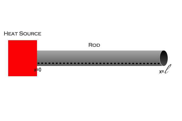
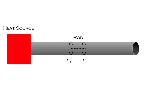
Let’s consider the segment of length 
![[x_{i}, ~x_{i}+\Delta x]=[x_{i}, ~x_{f}]](https://s0.wp.com/latex.php?latex=%5Bx_%7Bi%7D%2C+%7Ex_%7Bi%7D%2B%5CDelta+x%5D%3D%5Bx_%7Bi%7D%2C+%7Ex_%7Bf%7D%5D&bg=f0eeec&fg=222222&s=0&c=20201002)
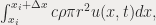
where 


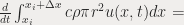
![c \rho \pi r^{2} \int_{x_{i}}^{x_{i} + \Delta x} u_{t}(x,t)dx = k \pi r^{2} [u_{x}(x_{i}+ \Delta x,t) - u_{x}(x_{i}, t)] + \pi r^{2} \int_{x_{i}}^{x_{i}+ \Delta x} f(x,t)dx](https://s0.wp.com/latex.php?latex=c+%5Crho+%5Cpi+r%5E%7B2%7D+%5Cint_%7Bx_%7Bi%7D%7D%5E%7Bx_%7Bi%7D+%2B+%5CDelta+x%7D+u_%7Bt%7D%28x%2Ct%29dx+%3D+k+%5Cpi+r%5E%7B2%7D+%5Bu_%7Bx%7D%28x_%7Bi%7D%2B+%5CDelta+x%2Ct%29+-+u_%7Bx%7D%28x_%7Bi%7D%2C+t%29%5D+%2B+%5Cpi+r%5E%7B2%7D+%5Cint_%7Bx_%7Bi%7D%7D%5E%7Bx_%7Bi%7D%2B+%5CDelta+x%7D+f%28x%2Ct%29dx&bg=f0eeec&fg=222222&s=0&c=20201002)
where 
Replacing 


where ![\alpha_{1}, \alpha_{2} \in [x_{i}, x_{f}]](https://s0.wp.com/latex.php?latex=%5Calpha_%7B1%7D%2C+%5Calpha_%7B2%7D+%5Cin+%5Bx_%7Bi%7D%2C+x_%7Bf%7D%5D&bg=f0eeec&fg=222222&s=0&c=20201002)
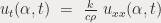
![u_{t}(\alpha,t)dx ~=~ \frac{k}{c \rho}[\frac{u_{x}(x_{i}+\Delta x,t)-u_{x}(x_{i},t)}{\Delta x}]+\frac{k}{c \rho}f(\alpha,t),](https://s0.wp.com/latex.php?latex=u_%7Bt%7D%28%5Calpha%2Ct%29dx+%7E%3D%7E+%5Cfrac%7Bk%7D%7Bc+%5Crho%7D%5B%5Cfrac%7Bu_%7Bx%7D%28x_%7Bi%7D%2B%5CDelta+x%2Ct%29-u_%7Bx%7D%28x_%7Bi%7D%2Ct%29%7D%7B%5CDelta+x%7D%5D%2B%5Cfrac%7Bk%7D%7Bc+%5Crho%7Df%28%5Calpha%2Ct%29%2C&bg=f0eeec&fg=222222&s=0&c=20201002)
Notice, however, we claimed our heat source was instantious. That is, for 


or,

Which, as the rod was laterally insalated, we claim that for the given system equation (2) is equivalent to,

Example of the Maximum Principle as a Physical Phenomena:
Consider the case where a rod is connected to a heat source as before. Consider the distribution of heat through the system after some time. We should expect a graph of heat as a function of position at some time 

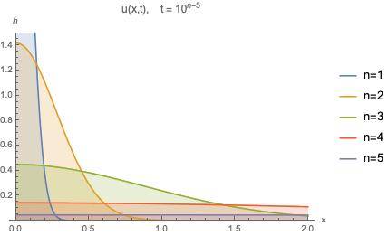
Here we can clearly see that for 
Similarly, let’s consider heat at some point 
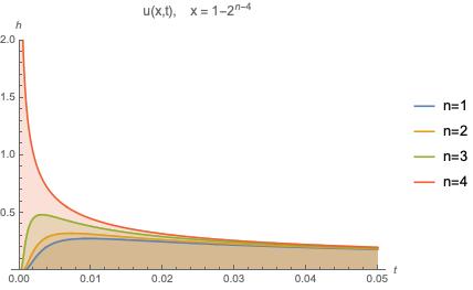
From this we can see that given 
For a copy of this:
For a copy of the notes used:
For a more “continuous” view of the evolution of heat…
…across the rod:
For a more “continuous” view of the evolution of heat…
…across time:
